
In the grounding testing industry, accuracy, transparency, and proper application of industry standards are essential to producing reliable results. Recent statements questioning the Smart Ground Multimeter (SGM) have created confusion about how the technology works and how it aligns with established testing practices. In the blog below, Dr. Sakis Meliopoulos, inventor of the Smart Ground Multimeter, addresses these claims directly and clarifies how the SGM uses current injection testing, advanced data processing, and operator-driven validation to support dependable ground performance testing.
Ground Performance Testing – Current Injection Test (CIT)
The Smart Ground Multimeter (SGM) has been described by others as a “numerical” method, implying that it does not provide actual test values. They assert that ground measurements should be made with a Current Injection Test (CIT), not with a “numerical method.”
The characterization of the SGM as “numerical method” is wrong; the SGM, as with any other measurement instrument, cannot make measurements with “numerical methods.” It injects a current into the ground under test, measures the resulting voltages, and processes the voltage data to obtain the ground impedance, touch voltages, step voltages, etc.
The SGM method is a current injection test (CIT) with the ability to inject up to 15 Amperes. It meets the requirements for ground impedance testing per IEEE Std. 81-2025. The SGM can use its own current injection circuit by running an overland conductor from the site to a temporarily installed current return electrode, or by using one overhead conductor in a de-energized distribution/transmission line (often not possible). Typically, the actual injected current is limited by the ground impedance of the injection circuit. The SGM’s injected current is an alternating current (positive/negative) to negate any galvanic voltages that may be present in the soil, and based on user selection, it comprises one single frequency or a range of frequencies to filter out site electrical noise.
The SGM measures the ground impedances at a user-selected frequency range: 0-250 Hz, 0-500 Hz, 0-1,000 Hz, or 0-2,000 Hz. The SGM results default to the 60-Hz power frequence; however, the user has access to the values measured at the entire frequency range that has been selected. The SGM software performs a number of procedures to (a) remove external interference, (b) perform error correction for induced voltages, and (c) perform calibration procedures to account for the exact placement of the current return probe and the voltage probes.
Describing the SGM as a “numerical method” is false. The CIT test method described in IEEE Standard 81 is the test method that is used by the SGM.
Test Operator Experience
Others have stated that some SGM testers operate with the belief that they do not need to follow grounding testing principles and interference avoidance techniques described in IEEE Standard 81 due to faith in the SGM’s abilities, causing concerns of whether data is valid.
Successful SGM use and all grounding test equipment and methods are dependent on the knowledge of the operators and their understanding of grounding testing principles, the relevant standards, and the specific equipment being used. No test equipment is magical. Unfortunately, in the grounding testing industry, many are not highly trained or aware of the interferences and challenges involved in this type of testing. Owners should spend time vetting prospective testing firms prior to engagement to ascertain their level of grounding testing experience. It is not the fault of the equipment if the user is not properly educated and does not have enough field test experience. Simply defaulting to the lowest-cost option can lead to issues, including incorrect test methods, bad data, and poor reports.
The SGM user’s manual and custom hands-on training class provide guidelines for modeling the grounding system, incorporating other nearby bonded or unbonded metallic/conductive objects, and routing test wires (overland) to minimize interference. It is also important to emphasize that these techniques simply reduce interference. The reality (physical laws) is that there will be interference regardless of the test equipment employed, and the results of the interference depend on the ground impedance of the system under test. For high impedance grounding systems, the interference effect is small in terms of error. For low impedance ground system, the effect of the interference could be a very high error. The SGM operator constructs the site grounding model, and the software then computes the interference and removes it from the measurements. This is a user-selected function; i.e., the user can turn the procedure ON or OFF and assess the results.
All grounding test equipment is subject to the laws of physics and real-world site challenges. The SGM provides the most data during and after testing, allowing a trained and knowledgeable operator to have the best chance at grounding testing success. The SGM provides a plethora of information during field testing, and the experienced tester can make adjustments to ensure that the test is successful and valid data is obtained.
Measurement Interference
Others have suggested that the SGM has limitations because it does not allow a user to interface with the measurement data as it is taken. This statement is incorrect.
This is where the SGM shines; it is the best instrument to perform and document the error correction methods to address the following common issues: (a) remove external interference, (b) perform error correction for induced voltages, and (c) perform calibration procedures to account for performance and the exact placement of the current return probe and the voltage probes. With the SGM software, the user can see the effect of each of these error-correction procedures. If the user prefers, he/she can use an alternative analysis program to compute error corrections independently and compare them with those provided by the SGM. The SGM method provides more data and interface than any other test equipment on the market.
Below is an example of measurements using the SGM, documentation of user interface information available during field testing, and all the error corrections applied to the measurements. The user can get the value of each correction at each frequency of the selected frequency range. This enables the user to compute these corrections with independent methods of their choice and compare them to what the SGM reports. Specifically, the user can see (a) the raw measurements, (b) the measurements after the external interference has been removed, (c) the measurements after the external interference and the induced voltages on the leads have been removed, and (d) the measurements after the external interference, induced voltages, and the correction for the placement of the probes and current return electrode have been removed.
Case Study
This example shows a high level of interference and harmonics. Note that the user has instant access (during the test) to the raw measurements and the data at each stage of the correction process. The user can obtain error-correction values for each frequency in the selected frequency range.
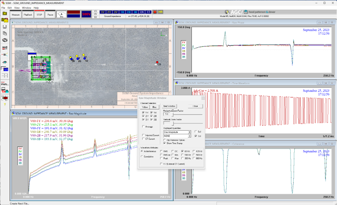
Figure 1: SGM User Interface During Test
Figure 1 illustrates a user selection of visualizations during a measurement; starting from the upper left corner and moving clockwise, the figure provides (a) probe arrangement, (b) raw measurement data converted into complex impedance – phase of the impedance, (c) time waveform of injected current, (d) coherence function that quantifies interference from power frequency and harmonics versus frequency, and (e) raw measurement data converted into complex impedance – magnitude of the impedance. Other user selections include: (1) measured probe voltage time waveform, raw measurements, (2) measurement data corrected for voltage probe resistance, voltage lead shunt capacitance, and (3) measurement data corrected from induced voltage on probe leads due to current return electrode current.
The middle right portion of Figure 1 shows a snapshot of the current waveform injected by the SGM source during testing. The full duration of the current is 571.2 milliseconds. It consists of a series of alternating positive/negative square pulses with randomly varying pulse width. The range of the pulse width is controlled so that the spectrum of the waveform is concentrated over a user-selected frequency range, specifically 0-250 Hz, 0-500 Hz, 0-1000 Hz, and 0-2000 Hz. The SGM source output can provide up to 500 Volts and 15 Amperes.
The lower right portion of Figure 1 provides the coherence function, a measure of the external interference noise contained in the six voltage measurements, over the user-selected frequency range (0-250 Hz in this example). Specifically, a coherence value of 1 at a certain frequency indicates that the measured probe voltage is nearly noise-free at that frequency, while a lower value indicates the presence of noise. Since noise is mostly occurring at DC, the power frequency and its harmonics, the coherence function typically has dips at 0 Hz, 60 Hz, 120 Hz, 180 Hz, etc. and is almost equal to 1.0 at all other frequencies. The coherence function is used to remove the measurements with high external noise. Coherence functions substantially below 1.0 at all frequencies indicate that the external noise is too high and cannot be removed. The user can modify the measurement setup in several ways to remove the external noise, as described in the SGM manual. The coherence functions provide a useful diagnostic to consider while conducting field measurements.
The lower left portion of Figure 1 shows the raw measurements converted into complex impedances: the magnitude of the impedance. The complex impedance is computed by first converting the measured probe voltages and the injected current measurements into phasors (using the FFT algorithm); then the impedance is computed as the ratio of the voltage phasors over the current phasors at each frequency. Note that the impedance is a complex number at each frequency, which is then converted into magnitude and phase angle. For simplicity, we refer to this data as the “raw transfer function.” The measurement process is repeated (typically 10 times), and the results are averaged. This averaging process substantially reduces noise at most frequencies except at frequencies with high noise concentration (i.e., DC, power frequency, and harmonics). The resulting curves contain error spikes at these frequencies. The display of the measured raw transfer function magnitude can be viewed during the field test.
The upper right portion of Figure 1 shows the raw measurements converted into complex impedances: the phase angle of the impedance. The complex impedance is computed by first converting the measured probe voltages and the injected current measurements into phasors (using the FFT algorithm); then the impedance is computed as the ratio of the voltage phasors over the current phasors at each frequency. Note that the impedance is a complex number at each frequency; the complex number is then converted into magnitude and phase angle. For simplicity, we refer to this data as the “raw transfer function.” The measurement process is repeated, and the results are averaged. This averaging process substantially reduces noise at most frequencies, except at frequencies with high noise concentration (i.e., DC, power frequency, and harmonics). The resulting curves contain error spikes at these frequencies. The display of the measured raw transfer function phase angle can be viewed during the field test.
Ground Impedance Reports (System Impedance and Mat Impedance)
The SGM is the only measurement system that can differentiate between system and mat impedance; there is no need to isolate and de-energize the site under test. Figures 2 and 3 provide the report of the measured grounding mat impedance and the system impedance versus frequency over the user-selected frequency range, as well as measurement error versus confidence level. The impedance values are generated based on a frequency-dependent model and the corrected measured probe transfer functions. The model includes the ground under test, voltage probes, current return electrode, voltage and current leads, and in the case of system impedance, the connected shield and neutral wires. Note that the statistical analysis shows the level of agreement between the actual measurements and the reported ground impedance versus frequency after all corrections have been applied, and the software evaluates the consistency between the measurements and the reported ground impedance.
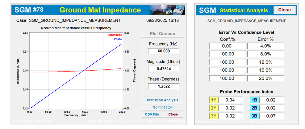
Figure 2: Mat Impedance
Figure 2 provides the report of the measured grounding mat impedance, as well as the statistical analysis. This result represents only the buried ground grid conductors of the substation, with the effect of the shield and neutral wires removed from the measurement. This is the measured value that is attempted with a Fall of Potential (FoP) test.
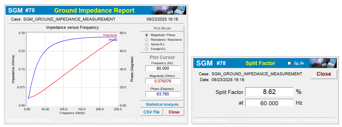
Figure 3: System Impedance
Figure 3 provides the report of the measured grounding system impedance, as well as the split factor. This represents the static conductor system ground and any neutrals, or other site grounding, in parallel with the buried ground grid conductors. The lower system impedance, as compared to the mat impedance, indicates the effect on the mat impedance due to its connection to the power network’s transmission and distribution ground system and any other grounds that are connected to and parallel with the ground grid.
Additional user interface screens are available, including:
- Average Soil Resistivity
- Measured Voltage Probe Time Waveforms
- Transfer Function Magnitude Corrected for Voltage Probe Response
- Transfer Function Magnitude Corrected for Power Frequency and Harmonic Interference
- Transfer Function Magnitude Corrected for Induced Voltage
- Estimated Transfer Function Magnitude
Key Takeaways
The SGM meets the requirements for ground impedance testing per IEEE Standard 81-2025. It uses a sophisticated, software driven test method that employs modeling and a current injection-based test (CIT) to provide validated grounding test data. The data can be viewed in real-time during testing and reviewed post-testing to improve the model and probe performance to validate results. No other grounding test equipment on the market can provide the level of interaction and data validation that the SGM provides. Successful SGM use requires training and extensive grounding testing knowledge; however, this is true with any ground test equipment and method. Other test equipment does not include diagnostics, and their lack of diagnostics does not increase confidence but rather should call into question the validity of their results. In most cases, testing is performed, and a value is produced with no analysis or interactive data to back up the results.